GEO381/550 Lecture note of
November 4th 2004 Dot Density Map
Dot density maps (dot maps)
Uses a dot to represent the
number of a phenomenon found within the boundaries of a geographic area
A way of illustrating the
spatial distribution of discrete objects
Best for representing
discrete value and counts
Designed to communicate
variation in spatial density
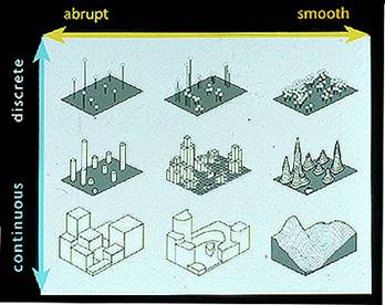
Figure 8.1b

When to use a dot density map
I. Phenomenon
Discrete phenomenon with
smooth variation
II. Data
Should be magnitude data:
total value rather than derived value
Example:
(1) Population density map
Let’s compare dot density
map with choropleth map… Any comment is welcomed!
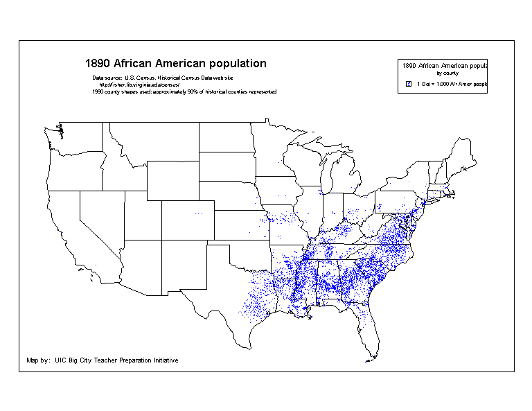
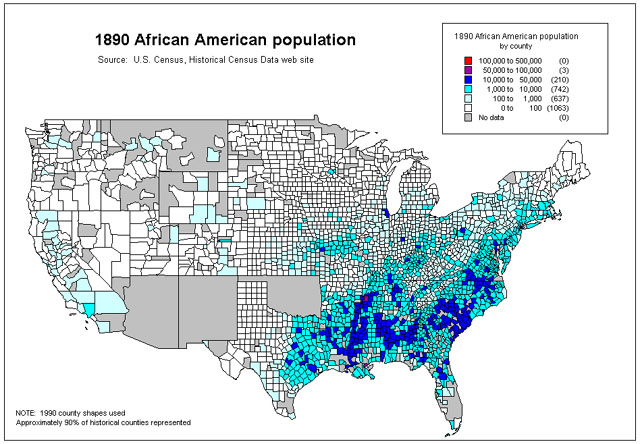
1890 1890
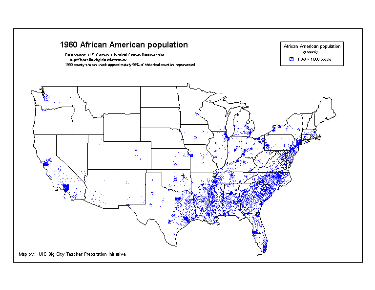
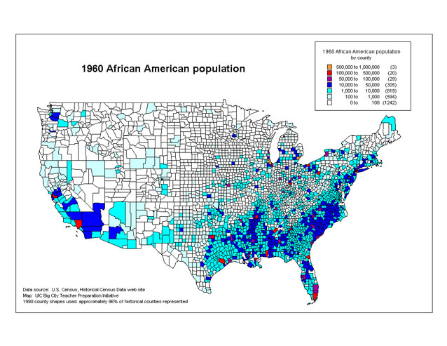
1960 1960
Source: African American
population by county
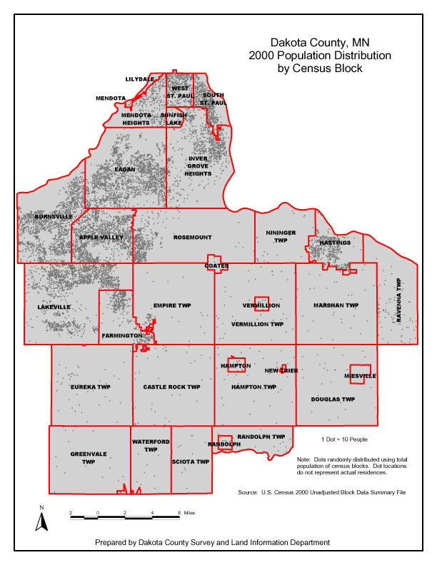
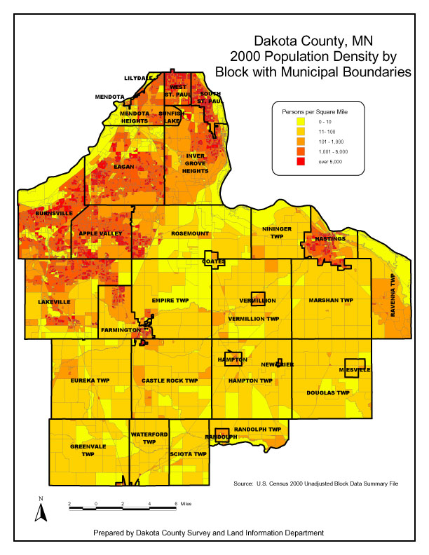
Source: South Dakota
population by census block
(3) Number of AIDS cases
Less abruptness is desirable
for change detection
Conceptual basis of a dot map
1. How it is constructed
Sprinkle dots so that each
dot represents magnitude which occupies varying size of territorial domain
Each dot can be thought of
as a spatial proxy for the real
phenomenon it represents
Dots are placed in the representative location
(the location where phenomena are mostly likely to occur), not in a precise
location (e.g. the location of shopping mall)
Each dot occupies
geographical space called dot polygons (or
territorial domains), which are not shown in the map
Figure 8.2
*Do not confuse dot
polygons with basic enumeration units
2.
How it is perceived
How many readers count the actual number of dots within each
enumeration unit?
The
dot map presents data at the ordinal level in the sense that readers judge that
there is more of the item in one place and less of it in another
In
other words, recovery of the original data may not be that important in this
mapping technique unless a map purpose is so
How it works
Suppose you make a dot map
of corn acreage in
(1) dot value
(2) dot size
(3) dot placement
Dot value
One dot represents what?
Upper bound: the value of
one dot should be smaller than the minimum value so that the dots in the lowest
enumeration area would not be eliminated (so <3,000) Too empty look is not
good
Lower bound: the value of
one dot should be larger than ?; it’s a matter of trial and error in the final
look. Choose a dot value such that the dots just begin to coalesce in the
highest enumeration area (i.e. densest part of the map). Too cluttered look is
not good.
Some other considerations:
a. Select a dot value that
is easily understood. For example, 50 is better than 49
b. Select a dot value so
that total impression of the map is neither too accurate nor too general
Dot size
Visual impression of varying
size of dots:
Small dots
------------------------------------------- Large dots
Visually accurate
visually crude
Changes on dot value and
size will produce very different maps (figure 8.7)
Dot placement
Place the dots where the
phenomenon is most likely to occur
You may need ancillary
materials to place dots properly
Don’t place dots in major water
bodies or urban areas – “limiting variables”
Try to place dots in
agriculture areas – “related variables”
Figure 8.3
What about computer mapping?
It’s randomly placed within
a basic enumeration unit…. so be aware of locational errors arising from random
placement!
Compare Figure 8.1b to 8.12
Random placement of dot
symbols leads to different maps (Figure 8.13)
So what can we do about it?
There seem to be two ways to
handle this:
(1) Do a manual work using
ancillary materials... hello?
(2) Use smaller enumeration
units! (see below: effect of size of enumeration units)
By the way, why does the
computer program prefer random
placement?
Figure 8.10 (acceptable and
unacceptable methods of dot placement)
(a) irregular pattern is superior to the regular one
(b)
boundary effects should be removed
Effect of size of enumeration
units
What if the data have been
collected in different enumeration units, say census block group, or county? What
are the consequences for using different areal units?
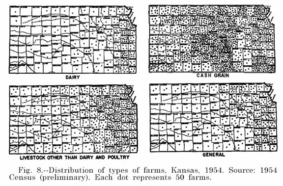
Figure 8.4 Accuracy
The smaller enumeration
units are in relation to overall size of the map, the greater will be the
degree of locational accuracy produced
The smaller enumeration units mean smaller dot polygons for
each dot, reducing the chance of locational error. As a result, greater
accuracy can be achieved
Look at the map above: number of farms in Kansas
Enumeration units (i.e. in which
scale data is aggregated) provide locational control
In relation to random
placement common in computer dot mapping, you can control locational accuracy
by using the data obtained from small enumeration units.
Other design
considerations
1.
Legend
Never
forget to include a statement indicating the unit value of the dot
Figure
8.11 Representative densities (low, middle, high densities) – visual anchors
Readers
perceive the map not by counting the dots, but by visually inspecting spatial
variableness at relative locations
2.
Map scale
Every
element (e.g. size of enumeration units, and dot size and value) should
harmonize with map scale.
3.
Map purpose
For
example, when recovery of original data (i.e. want to know actual number of
dots within enumeration units) is important, some visual considerations should
be exchanged for accuracy (e.g. do not use coalescing dots)
Advantages and disadvantages of dot mapping
Advantages:
- Intuitive (e.g.
Figure 8.1b)
- Reveals overall pattern of the spatial
distribution of the discrete geographic phenomena with smooth variation
- If dots are manually placed by taking into
account the distribution of functionally related phenomena, the map can
reveal a meaningful pattern.
Disadvantages:
- Difficulty in estimating density
- Dots may be interpreted as representing a single
instance of the phenomenon at a particular location
- If dots get too dense, it is impossible to
recover the original data in most cases
Next
time: Cartogram (READ CHAPTER 11)