Geo520 Lab 2: File Formats in TransCAD

Lab2 of Geo520, Spring 2005

TA : Julie Hwang

Lab 2. File Formats in TransCAD

Working with Table and Spatial Overlay

Objectives

[1] Understand file formats used in TransCAD

[2] Be familiar with operations for manipulating tables

[3] Perform spatial overlay between layers

File Formats in TransCAD

______ Open TransCAD. When TransCAD quick start window pops up, click OK. When the File Open window pops up, look at the Files of type drop-down list at the bottom. The drop-down list contains file formats available in TransCAD. Some are internal to TranCAD, and others are not. In this lab, we’re focusing on its own special file formats.

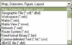
Maps, Dataview, Figure, and Layout

Documents displayed in different windows (eg. Map, Dataview) can be saved as a separate file as listed below. Do you know how to save it?

File Extension	Application
.map	TransCAD Map
.fig	TransCAD Chart or Figure
.dvw	TransCAD Dataview
.lay	TransCAD Layout

To support Map and Dataview, two types of files (geographic file and attribute file) are fundamental to a database in TransCAD.

Geographic files

TransCAD’s internal geographic files come in two formats:

· Compact Geographic Database: A compact, read-only format that displays very quickly. This type of geographic database contains a file with extension .cdf and some other affiliated files.

· Standard Geographic Database: An editable format that takes more space and displays less quickly. This type of geographic database contains a file with extension .dbd and some other affiliated files.

Attribute files (tables)

TransCAD can read many formats of tabular files. For example, it can read .dbf file, comma-delimited text, fixed-format text, fixed-format binary, and matrix (with extension .mtx) and dataview files (with extension .dvw).

Other supported file formats

There are still other file formats to support other extended TransCAD documents, such as Network and Route systems. We will leave those (matrix, network, and route system) to future lab discussions.

File Extension	Data Model
.mtx	Matrix
.net	Network
.rts	Route system

Practice #1: Open attribute files

______ Create a map named Flintbury_lab2 by adding two layers FL_ZONE.CDF, and FL_ST.CDF located in the Tutorial Dir. You can add multiple layers into one map by using shift key in the File Open windows instead of adding one by one by choosing Map-Layers: Add Layer button.

______ This time you want to view an attribute file that contains additional information of the street layer. Open FL_STDATA.BIN by clicking and choosing Fixed-format Binary (with an extension .bin) from the Files of type drop-down list.

______ Browse for the fields in the opened attribute file.

Practice #2: Compute statistics of attribute files

______ Suppose you want to know the average operation speed of streets in this study area. Make sure FL_STDATA.BIN is an active window. Choose Dataview–Statistics, and then save the output binary file in your home directory.

______ Check the minimum, maximum, mean, and standard deviation of [OPER SPEED]. Ensure that the operation speed in this area is 36.56 on average within the range between 10 and 65.

______ You might want to save this file as other file format such as .dbf or .txt for future use. That way, you can access this file with other softwares (such as fox pro, or text editor). Use File–Save As… while a davaview is open.

Parctice #3: Join two tables with a common field

______ Compare attributes of street layer (FL_ST.CDF) with those of the binary file (FL_STDATA.BIN). Sort each table by ID (or STREET ID) field by choosing Dataview-Sort…. (right-mouse click with the selection of the field will do the same) You may see they share the common field by looking at ID and the number of records shown in the status bar in the bottom left.

______ Suppose you want to join Street layer to an attribute file. Make the dataviews of Flintbury Streets an active window. Choose Dataview-Join… (or ) . The following window will pop up.

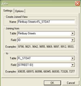
______ Make sure you choose the appropriate table and field in the Join window as shown above. Click OK. Joined table view will pop up.

Practice #4: Create a thematic map based on the joined attributes

______ Since the street layer is joined to an attribute table, now you can create a thematic map based on joined attributes. Make the map of Flintbury streets the active window. Choose Map-Scaled symbol Theme…(or ) when a street.layer is made active layer in the map.

______ When Scaled Symbol Theme window pops up, you can see the joined attributes in the Field drop-down list. Choose [EST VOLUME] from the Field drop-down list.

Practice #5: Use formula fields

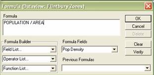
You may want to know the attributes that are calculated from existing fields. For example, if you want to know population density when you have the fields [Population] and [Area], you can easily obtain the value of population density ([Population] / [Area]). In TransCAD, there are two different options for doing this. Dataview-Formula Field… (Practice #5) and Dataview-Modify Table… (Practice #6). With the first one, editing results are not saved (only displayed in dataview) whereas the second one saved the results permanently in the file.

______ Open the dataview of the layer Flintbury_Zones. Choose Dataview-Formula Fields…. Type the appropriate values in the Formula text box using Formula Builder. Remember to type in the name in the Formula Fields as well (Don’t be confused as it looks like drop-down list - you can “actually” type in like textbox). Click OK.

______ Now you will be able to create a thematic map based on formula field. Create a population density map. (This can be done using color-map.) If you want to remove a scaled-symbol map of street, click Remove button in a scaled-symbol map dialog box (make sure street layer is active then).

______ Remember formula fields you created would not be saved if you close files without saving them as other files.

Practice #6: Modify tables

______ To practice this part, you need to copy the geographic files (FL_ZONE.*) to your home directory because it will modify the files permanently. Alternatively, use Tools-Export… when the geographic file you want to copy is active. Then choose compact geographic file in To drop-down list.

______ Open the geographic file FL_ZONE. Open its dataview. Choose Dataview-Modify Table…. The Modify Table window will allow you to add, drop the fields as well as change the order of fields.

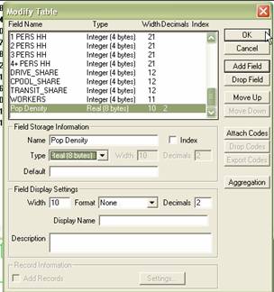
______ Click Add Field button. Then Name the field as well as the type of the field (Make sure you set Real for the Type drop-down list. Otherwise the value under the decimal point will be truncated). Click OK.

______ In the dataview, select the field bar named say [Pop Density] at the top, then right-click in the mouse. Choose the Fill… in the menu. Check the Formula among check boxes when the Fill window pops up.

______ Do the same as you did in formula field in the previous practice when the Formula window pops up.

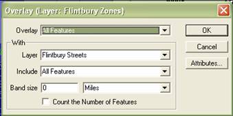
Practice #8: Spatial overlay

What if you want to know the average estimated traffic volume by zone? How can we do that? It’s not like table join, rather we are going to join two tables (of zone and street layers) based on their spatial relationship. Now we are going to overlay zone with street layer. To perform spatial overlay, you need to set the working layer (for which you want to calculate the data) and the reference layer (whose data you want to tally). In this practice, FL_Zone is the working layer, and FL_ST is the reference layer because you want to assign attribute values in a street layer to a zone layer.

______ Make the layer FL_Zone active. Then choose Tools-Geographic Analysis-Overlay… When Overlay window pops up, set the reference layer as shown below. (Make sure Flintbury Streets layer contains the joined attributes in it)

______ Save a bin file in your home directory. Browse through a dataview that pops up. For example, resulting [EST VOLUME] value 929742 of zone ID 18409 (first record) in this dataview indicates sum of [EST VOLUME] of street features contained in a zone feature with the ID. Also note [Avg EST VOLUME] is [EST VOLUME] / number of street features that lie in each zone feature.

______ Create a choropleth map showing the average estimated volume by zone (you have to choose the field [Avg EST VOLUME] in the Field drop-down list in the Color Map windows)

Assignments (due at the beginning of next lab):

Use the geographic files RI_CNTY, and RI_HWY from the tutorial directory (copy those files to your home directory). Suppose you are asked to make a presentation about highway characteristics and traffic in each county of Rhode Island. Your presentation should include a map of per capita highway traffic in each county as well as summary statistics of highway layer.

To obtain per capita highway traffic in each county, you should (1) overlay county with highway, (2) compute (AB TRAFFIC + BA TRAFFIC) / POPULATION, (3) make a color map. For summary statistics of highway, follow Practice #2. (AB TRAFFIC means traffic count for each road segment in one direction; BA TRAFFIC means traffic count for each road segment in other direction)