Geog 460: GIS Analysis
11/14/05
Spatial Interpolation
Mapping rainfall…
You begin with location of 36
climatic stations

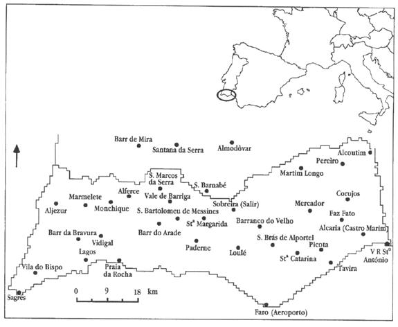
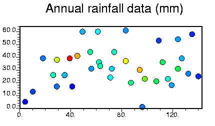
Input> you collect/compile
annual rainfall data for each station
Output> you produce two
maps
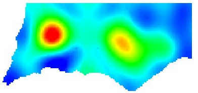
Rainfall map A
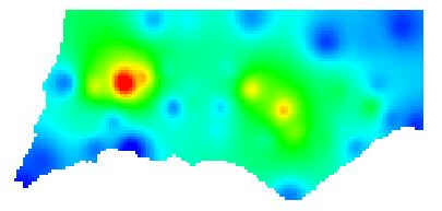
Rainfall map B
Operation>
Maps differ because they
employ different operations, here spatial interpolation methods (e.g. A uses
Inverse Distance Weighted or IDW and B uses Kriging).
Different spatial interpolation methods yields
different results.
Image source:
http://www.geovista.psu.edu/sites/geocomp99/Gc99/023/gc_023.htm
What is spatial interpolation?
Spatial interpolation is the
procedure of estimating the value of properties at unknown locations based on
measured values at sample locations
In other words, spatial
interpolation is used to derive “continuous” surface at all locations from
values at sampled locations
It requires some assumption
of the continuity and distribution of surface (e.g. spatial autocorrelation)
Why spatial interpolation?
1. Need for inference given
constraints
It is desirable collecting
sample values at as many locations as possible (because it is more accurate),
but it is expensive. Accurate “estimation” of values at unknown locations may
be quite difficult, but valuable.
e.g. Submarine cruising around “estimated” topography of
ocean floor
e.g. mining industry: initial feasibility study
2. Visualization
Visually more attractive,
more amenable to decoding when variation in attribute values is smoothed out
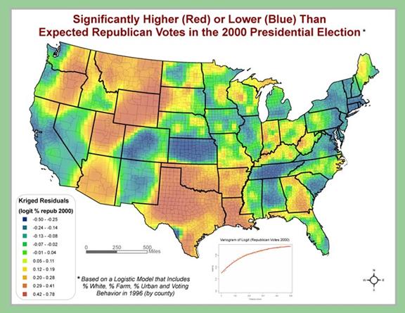
Image source: www.zevross.com/mapplot/repub.jpg
Spatial interpolation methods
Inverse Distance Weighted (IDW)
IDW estimates cell values by averaging
the values of sample data points in the vicinity of each cell. The closer a
point is to the center of the cell being estimated, the more influence, or weight, it has in the average process.
Values are estimated by

Where zj
is the estimated value for the unknown point at location j, dij
is the distance from known point I to unknown point j, zi
is the value for the known point i, and j is a
user-defined exponent.

Image source: Bolstad 2005
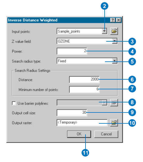
You have options for choosing
the weighting exponent n and the
number of points i considered for estimation.
Q.
consequences of different parameter values?
When a larger n is specified the closer points become
more influential
When a large number of sample
points i
tends to result in a smoother interpolated surface
You should know the impact of
varying values of these parameters as you will be asked to choose the value
when you use GIS. The following image shows ArcGIS
Spatial Analyst
There are two kinds of spatial
interpolation methods: one is deterministic and the other is stochastic.
Stochastic methods incorporate the concept of randomness. Deterministic methods
do not use probability theory. Kriging is a
statistically-based estimator of spatial variables.
Kriging
In a generalized form,
spatial interpolator can be seen as the weighted sum of data. In IDW, the
weight depends solely on the distance (or its power function) to the prediction
location.
In Kriging,
the weights are based not only on the distance, but also on the spatial
structure of data. The model of spatial dependence is built first, and then
values at unsampled points can be predicted from the
model. Model building is similar to regression analysis, where the weight is
determined such that variance is to be minimized. The model building begins
with variogram.
Variogram (a.k.a. semivariogram)
It summarizes spatial
autocorrelation (or spatial dependency) based on observed values
In Variogram,
x-axis represents the distance between points (a.k.a. lag distance) (let’s
denote this as h), and y-axis represents semivariance.
Semivariance  where n is
the number of points, za
is the elevation in location a, zb is the
elevation in location b.
where n is
the number of points, za
is the elevation in location a, zb is the
elevation in location b.
Semivariance measures how elevation values are similar to the
values in neighbors. Larger semivariance values mean
that values are less similar while smaller semivariance
values means that values are more similar to each other. Thus, semivariance is a measure of the interdependency of the elevational values based on spatial proximity.
The empirical semivariance is plotted against lag distance as shown
below.
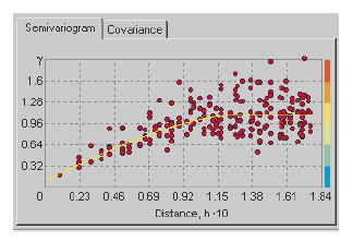
Then you
choose theoretical model into which the empirical variogram
is fitted. The fitting process attempts to minimize the deviation from the
observed (empirical) value to theoretical model.
Variogram in theory would look like this. It has three
elements: sill, range, and nugget. Sill is the value of semivariance
where semivariance levels off. Range is the lag
distance where sill is reached. Nugget is the intercept with y-axis.
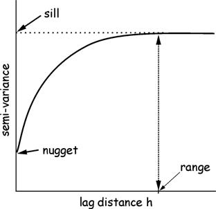
When the distance between
samples is small, the semivariance is also small.
This means that the elevational values are very
similar because of their close spatial proximity. As lag distance between
points increases, there is a rapid increase in the semivariance,
meaning that the spatial dependencey of values drops
rapidly.
Eventually, a critical value
of lag known as the range occurs, at which point the variance levels off and
stays essentially flat. Beyond the range, the distance between points makes no
difference. This information gives us a measure of what neighborhood needs to
be applied.
Now we can summarize that spatial
structure of the data can be decomposed into three components.
(1)
Global trends
(2)
Local variations
(i.e. spatial autocorrelation)
(3)
Random term
Using analogy, when you’re
hiking (let’s say you’re climbing), the elevation goes up. That is the trend.
While you’re hiking, you noticed that slope is going up and down at the local scale.
That is local variation. Sometimes you tip over boulder, which can be seen as a
random term.
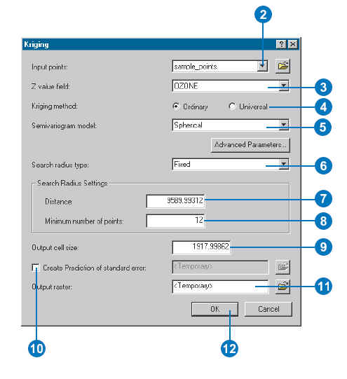
Kriging reports standard error. The report will show how well
your empirical model fits well into the theoretical model (see the number 10
below).
There are ways to assess
accuracy of interpolation derived from deterministic method: cross-validation
Other interpolation method
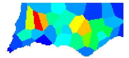
Proximal method (or nearest neighbor method)
Unknown values are assigned
to the value same as nearest neighbor
Nearest neighbor can be
derived based on Thiessen polygon
(a.k.a. Voronoi diagram)
Yields abrupt change in the
boundary
Can be used if you want to
approximate the unknown boundary of point data (e.g. trade area) under the
assumption of same magnitude of influence
Spline method
It tries to fit observed
value to mathematical function (such as polynomial function)
Good for representing nice
smooth variation
Used to draw smooth contour
from TIN
These methods (proximal, and spline) are deterministic